5 Population Ecology

Thousands of bird species breed and reproduce in North America. Some, like the American Robin (Turdus migratorius), are widespread, and can be found building nests and raising their young in every state of the USA, several Canadian provinces, and many locations in Mexico. Others, like Kirtland’s Warbler (Setophaga kirtlandii) breed almost entirely within a single state (Figure 5.1); a few, like the Cozumel thrasher (Toxostoma guttatum) and Socorro mockingbird (Mimus graysoni) are found only on single small islands. Population ecologists study what determines the occurrence and abundance of species in space and time: their geographic ranges, population sizes and densities, and what factors result in them being so rare or common.

Population ecology is the science of population dynamics in space and time

Ecology is often defined as the study of the distribution and abundance of organisms. Population ecology is the branch of ecology that works to understand the patterns and processes of change over time or space for populations of a single species. A species is typically defined as a group of organisms capable of interbreeding. For some species, all of the members of the species occur in the same geographic area and could potentially meet and interbreed during their lifetimes. Most species, however, can be divided into geographically separate populations. Individuals within a single population are likely to interact and perhaps inter-breed, while those from different populations will only come into contact if there is long-range movement between the populations (dispersal).

Populations can be described by their size, density, or spatial extent

One species that currently consists of a single population is the Kirtland’s warbler (Setophaga kirtlandii), a North American songbird. Almost all members of this species occur in the northern part of the state of Michigan in the United States (Figure 5.1). In contrast, the Spotted Owl (Strix occidentalis) is a species with many distinct populations throughout the western United States, southern Canada, and central Mexico.

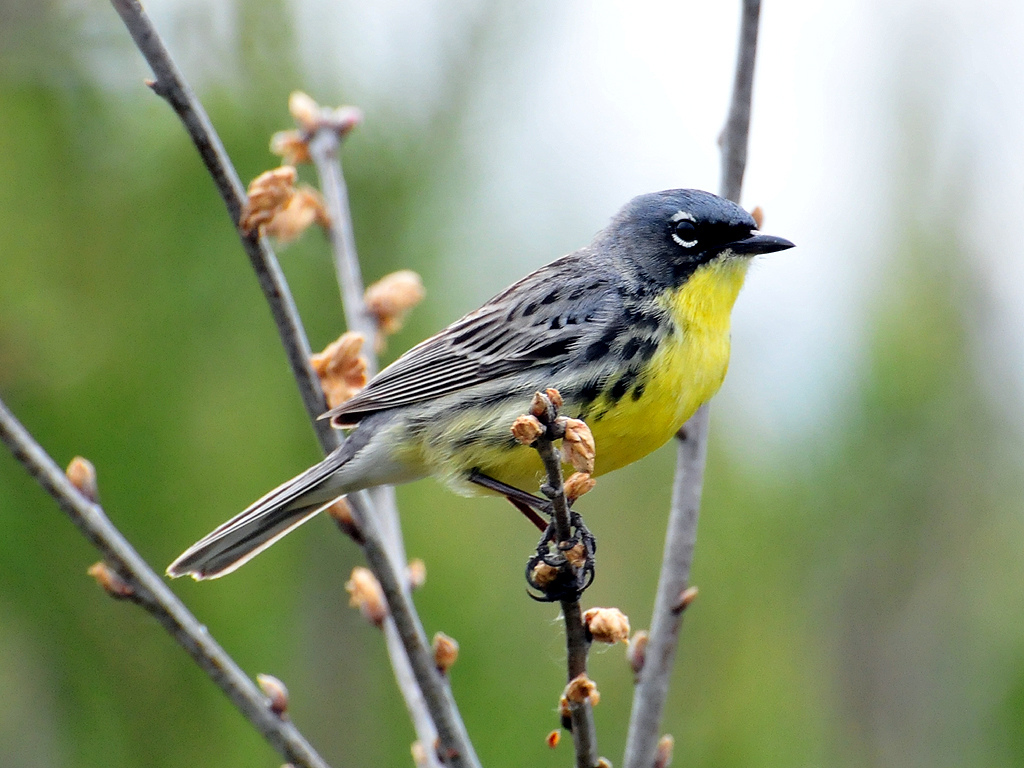
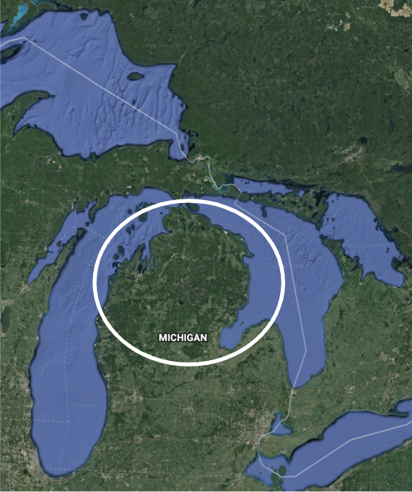
Figure 5.1: Left: “A male Kirtland’s Warbler Setophaga kirtlandii in a forest in Michigan, USA” by Jeol Trick is licensed under CC BY 2.0. Right: Core habitat area of Kirtland’s Warbler. Source: Google Earth: https://bit.ly/3ofgDK1.

For both species and populations, patterns of distribution and abundance can be considered in several ways. These include:

• Size: How many total individuals there are?
• Density: How many individuals per unit of area?
• Dispersion: How are individuals in a population arranged spatially relative to another? Do they occur in clumps or are they evenly spread apart?
• Occupancy: Does a species or member of a population occur in a given habitat, or is it absent?
• Population distribution: Where does a population occur in space?
• Geographic range: What are the furthest geographic limits of where a species occurs?

In addition to static characteristics of size and distribution, populations are dynamic and fluctuate based on a number of factors: seasonal and yearly changes in the environment, natural disasters such as forest fires and volcanic eruptions, and competition for resources between and within species. To study these many facets of a population’s biology, ecologists use both systematic field observations to determine its current status, and mathematical tools to characterize how it responds to changes in the biotic and abiotic environments.

Population size is the number of individuals in a population

Population size is the actual number of organisms in a population. This is often of great interest to biologists – especially those working in forestry, wildlife management and conservation – and most of our basic population models work with population sizes. A complete census is one way to determine population size and entails counting each individual present within the population. This occurs in some well-studied populations, such as the Kasekela population of chimpanzees in Gombe National Park, Tanzania (Pusey et al. 2008), and the Seychelles Warbler on islands in the Indian Ocean off the coast of East Africa (Burt et al. 2016).

Although it is the most accurate methodology, counting every individual in a population can be difficult, if not impossible. In most cases ecologists can only attempt to estimate the population size by using well-designed field studies and statistics. Indeed, some population ecologists specialize in developing mathematical and statistical models to accurately estimate population size. Often, however, we do not have good estimates of the size of a population itself, but factors that should be correlated with the population size, such as the number of animals harvested by hunters or trapped by ecologists or the density of dung found during a survey.

Data that we think correlates with actual abundance constitutes a population index. Index data are cheaper to collect than the data needed for formal estimates of population size, but can be biased and provide an inaccurate sense of the status of a population (Stephens et al. 2015). Ideally, an index should be validated by checking its correlation with rigorous estimates of population size. For example, the abundance of large mammals such as lions, elephants and tigers is frequently indexed by the frequency of their tracks or scat. To determine the reliability of an indirect measure of population size, Belant et al. (2019) compared an index based on lion tracks to a formal estimate of population size. Unfortunately, the commonly used index of lion abundance based on their tracks overestimated abundance.

When species become endangered researchers often try to determine – or at least estimate – the number of individuals surviving. For example, with only approximately 4000 individuals, Kirtland’s Warbler is the rarest species breeding in the continental United States and was considered critically endangered throughout most of the 20th century. Researchers therefore worked each spring to determine as best as possible how many male warblers had established territories and were trying to attract mates.

Species that are economically important or are central players in ecosystem functioning are also often monitored intensively. Since the middle of the 20th century the abundance of Wildebeest (Connochaetes taurinus) in the Serengeti ecosystem of East Africa has been intensively monitored by aircraft (Figure 5.2). The population was considered to be small in the 1960s when it numbered around 250,000, but by the 1990s had grown to over 1 million (Mduma et al. 1999).

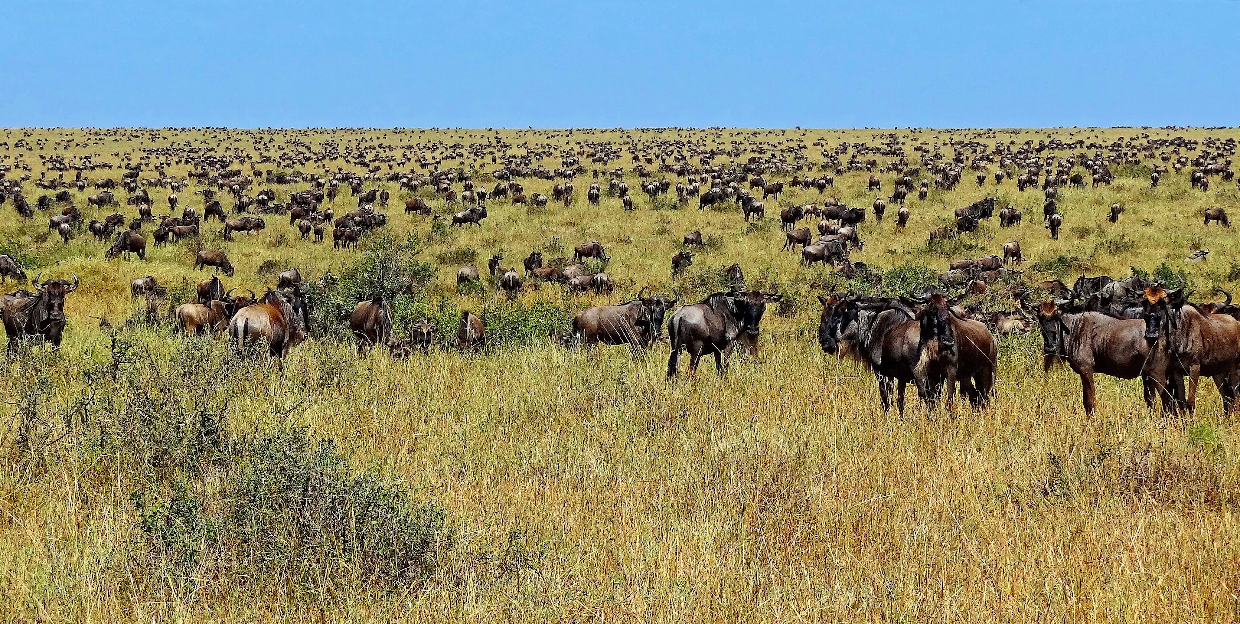
Figure 5.2: Wildebeest in Maasai Mara. Photo by Bjørn Christian Tørrissen, http://bjornfree.com/galleries.html.

Population density is the relative abundance of an organism

While population size is a total count of individuals, population density is how many individuals occur in a given area of space. It is therefore a measure of relative abundance. For animals and trees, this is often the estimated number of animals per hectare (a hectare is 100 m by 100 m, or 2.47 acres). For plants, insects, and other smaller organisms this is often the number per square meter.

How do populations change?

Changes in population size over time and the processes that cause these to occur are called population dynamics. How populations change in abundance over time is a major concern of population ecology, wildlife ecology, and conservation biology, and is related to questions asked in evolutionary biology. The processes and mechanisms that drive population change are varied and include intraspecific competition with members of the same population, interspecific competition between species, the availability of food or other resources, extreme weather, inbreeding, predators or parasites.

Populations are dynamic and frequently change size, density, or spatial extent

We can consider changes in populations from multiple angles. For example, Kirtland’s Warbler (Setophaga kirtlandii) in North America is currently:

• Increasing in the overall number of individuals (population size).
• Increasing in the number of occupied habitat patches (occupancy).
• Increasing in the geographic area it occurs in (population distribution and species range).

Importantly, since the warbler prefers a certain density of Jack Pine, its density within an occupied habitat also changes. Jack Pine stands are naturally prone to burning in forest fires, and are also logged for timber. As the density of trees changes due to these disturbances, the density of warblers changes. After a fire or logging there are few if any mature pine trees and therefore few warblers. Approximately five years after seedlings have sprouted and grown up to be the proper size, the density of warblers can increase. When pine forests get too old habitat conditions are not ideal for the warbler and their abundance declines.

Many studies of population growth focus on changes in population size

Discussions of population dynamics often center on changes in population size over time. Changes in population size are often displayed in a time series graph with time on the x-axis (usually in years) and population size (N) on the y-axis. General patterns of population dynamics in terms of population size include:

• Growth: Growing larger than the current size (Snail kites: Figure 5.3 Panel C)
• Decline: Decreasing in abundance (Elk: Figure 5.3 Panel B)
• Stability: Staying approximately the same size over time (Wolves: Figure 5.3 Panel C)
• Recovery: Stability or growth following a period of decline. (Impala: Figure 5.3 Panel D)
• Extirpation (local extinction): Decline of one or more populations of a species to 0 (Kirtland’s Warbler, Figure 5.4 Panel A)
• Extinction: Decline of all members of a species to 0 (Northern White Rhino, Figure 5.4 Panel B)
• Cycles: repeated patterns of growth followed by decline (Lynx: Figure 5.4 Panel C)

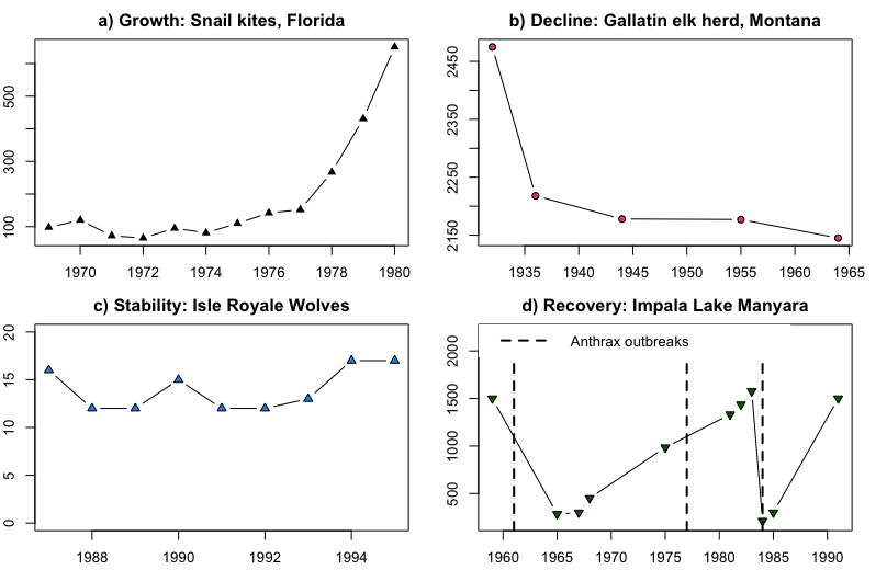
Figure 5.3: Common patterns of population change. The x-axis in all panels is the year and the y-axis is the number of individuals. a) Growth in a Florida Snail Kite (Rostrhamus sociabilis) population from 1970s to 1980s (Sykes 1983); b) Decline of the Gallatin, Montana herd of elk (Cervus canadensis) from the 1920s to 1960s (Peek et al. 1967); c) Stability of the Isle Royale, Michigan pack of wolves (Canis lupus) in the 1980s and 1990s (Peterson et al. 1998); d) Recovery after population crashes in the Lake Manyara National Park, Tanzania herd of impala (Prins and Weyerhaeuser 1987).

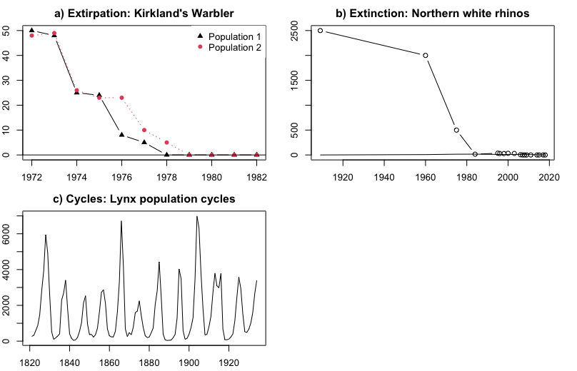
Figure 5.4: Common patterns of population change. The x-axis in all panels is the year. a) Decline to extirpation (local extinction) of Kirtland’s Warbler in two populations (Probst 1986). The y-axis is the number of singing males; b) Decline to global extinction of the Northern White Rhinoceros (Ceratotherium simum cottoni), one of two subspecies of White Rhinos (Smith 2001, Emslie 2012). The y-axis is the total number of rhinos in the wild. c) Repeated cycling of the Canada lynx (Lynx canadensis; Campbell and Walker 1977). The y-axis is the number of lynx trapped, an index of population size.

Over the course of many years, a single population can display many of these dynamics. For example, Kirtland’s Warbler populations were monitored by determining the number of males defending territories in their summer breeding habitat in the Great Lakes region North America, primarily Michigan. There were about 500 males with territories in the 1950s (Figure 5.5). The following changes occurred over the next 50 years after the species began being protected by the Endangered Species Act (Kepler et al. 1996):

• Decline over the course of the 1960s to ~200 territories.
• A period of stability at ~200 territories from 1975 to 1990.
• Steady growth to >2500 from 1990 through 2020.

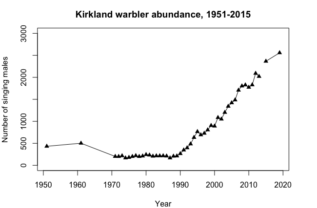
Figure 5.5: Number of singing Kirtland’s Warbler (Setophaga kirtlandii) males, 1950 to 2020.

Models can be used to understand and predict population dynamics

Researchers who study population dynamics often use mathematical models to describe and predict population dynamics and understand what factors are driving those changes. For example, if there are 2500 Kirtland’s Warblers in Michigan this year, can we predict how many will be around next year, or 10 years from now? Due to its small population size the Kirtland’s Warbler was listed as an Endangered Species in 1967. In 2019 it was de-listed and now is considered “Near-threatened.” Ecologists are very interested in using models to predict how large the Kirtland’s Warbler population will be in the future, and what factors cause it to increase and decrease (Brown et al. 2019). In the next chapter we will explore the conceptual and mathematical tools ecologists use to understand population dynamics and predict their future trajectories.

Biotic interactions and abiotic conditions limit the sizes of populations

Population dynamics can be regulated in a variety of ways. These are grouped into density-dependent factors, in which the density of the population at a given time affects growth rate and mortality, and density-independent factors, which influence mortality in a population regardless of population density. Note that in the former, the effect of the factor on the population depends on the density of the population at onset. Conservation biologists want to understand both types because this helps them manage populations and prevent extinction or overpopulation.

Density-Dependent Regulation

Most density-dependent factors are biological in nature (biotic), and include predation, inter- and intraspecific competition, accumulation of waste, and diseases such as those caused by parasites. Usually, the denser a population is, the greater its mortality rate. For example, during intra- and interspecific competition, the reproductive rates of the individuals will usually be lower, reducing their population’s rate of growth. In addition, low prey density increases the mortality of its predator because it has more difficulty locating its food source.

An example of density-dependent regulation is shown in Figure 5.6 with results from a study focusing on the giant intestinal roundworm (Ascaris lumbricoides), a parasite of humans and other mammals (Croll et al. 1982). Denser populations of the parasite exhibited lower fecundity: they contained fewer eggs. One possible explanation for this is that females would be smaller in more dense populations (due to limited resources) and that smaller females would have fewer eggs. This hypothesis was tested and disproved in a 2009 study which showed that female weight had no influence (Walker et al. 2009). The actual cause of the density-dependence of fecundity in this organism is still unclear and awaiting further investigation.

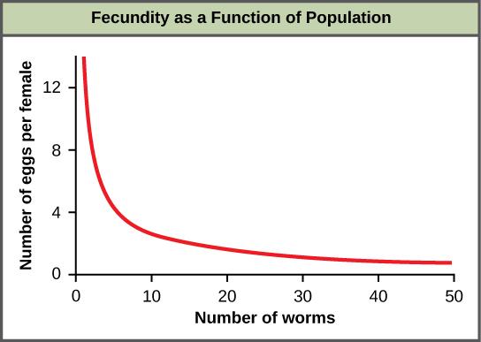
Figure 5.6: In this population of roundworms Ascaris lumbricoides, fecundity (number of eggs) decreases with population density (Croll et al. 1982).

Density-Independent Regulation and Interaction with Density-Dependent Factors

Many factors, typically physical or chemical in nature (abiotic), influence the mortality of a population regardless of its density, including weather, natural disasters, and pollution. An individual deer may be killed in a forest fire regardless of how many deer happen to be in that area. Its chances of survival are the same whether the population density is high or low. The same holds true for cold winter weather.

In real-life situations, population regulation is very complicated and density-dependent and independent factors can interact. A dense population that is reduced in a density-independent manner by some environmental factor(s) will be able to recover differently than a sparse population. For example, a population of deer affected by a harsh winter will recover faster if there are more deer remaining to reproduce.

Contributors and Attributions

Modified from the following sources:

Ecology for All! By LibreTexts, Chapter 9.1 and Chapter 9.3 licensed CC BY-NC-SA

Additional references and citations from the above sources can be found in References in the backmatter.

5. Population Ecology is shared under a CC BY-NC-SA license